1. The CONCAT function
The CONCAT function was formerly known as CONCATENATE.
The difference is, with the new CONCAT function you can select a range of cells, e.g. =CONCAT(B1:B4), whereas with the old CONCATENATE, you had to select each cell individually, e.g. =CONCATENATE(B1,B2,B3,B4).
In the example given below, the first, middle and last names are combined in Column D by entering =CONCAT(A2,” “,B2,” “,C2)
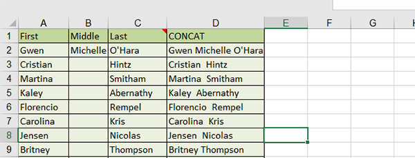
Using the CONCAT function to merge First, Middle and Last Names into one cell.
2. The TEXTJOIN Function
The new TEXTJOIN function is the alternative to the CONCAT function.
You can specify that you want to separate each value with one of the delimited characters, such as tabs, semicolons, commas, spaces or other types of characters. You can also specify which empty cells you wish to exclude within the range you have selected.
For example, you may have a list of first, middle and last names in separate columns and you wish to combine these ranges including a delimiter you specify, such as =TEXTJOIN(” “,,A2,B2,C2) in column D, example given below.
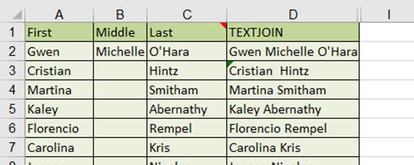
Using TEXTJOIN to combine First, Middle and Last Names together in one cell.
3. MINIFS And MAXIFS Functions
With the new MINIFS/MAXIFS you can return the lowest or highest value over multiple criteria in two or more columns. This is different to the existing MIN/MAX functions, which only return the smallest/largest number in a set of values from one set of data in a column.
In the example given below, you want to find the highest value (MAXIFS) if the Area is North (column A) and the Category Savoury (Column C). So, for e.g. =MAXIFS($G:$G,$A:$A,$T6,$C:$C,$U6)
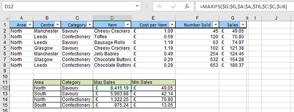
Using MINIF and MAXIF functions to work out the highest and lowest sales for various items.
4. IFS Function
You’ve probably encountered situations where you were required to perform more than one series of logical tests using the nesting IF function — having one formula inside another.
The great news is that we can now say goodbye to nesting IF functions and introduce you to the IFS function, which is a new way of creating a nested IF. The simpler structure makes it easier and quicker to create complex nested IFS.
In other words, the IFS function avoids nesting the number IF function in the calculation.
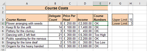
Using the IFS function to figure out whether a course can go ahead or not.
In the example given above, a training centre needs to know whether a course will run by creating an IFS formula in column E to say whether they have the right number of delegates. Over 15 is “too high”, between 3 and 15 is “OK” and less than 3 is “too low” e.g. =IFS(B4<$H$4,”Too Low”,B4<=$H$3,”OK”,TRUE,”Too High”)
5. SWITCH function
If you are struggling to work with IFS, nesting IF functions or VLOOKUP/HLOOKUP functions, this new SWITCH function may be the one for you.
SWITCH allows you to compare several different values and lookup for the exact match. As the SWITCH function will only find an exact match, there is no logical test like with an IF.
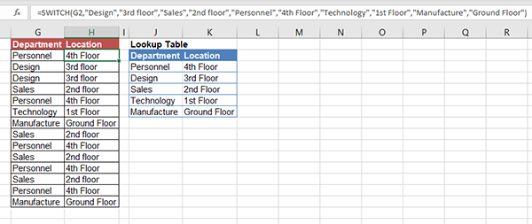
Using the SWITCH function to display the location of different departments.
In the example above, you are looking up the location of different departments.
For instance, if the department is “Personnel”, its location will be on “4th floor” e.g. =SWITCH(G2,”Design”,”3rd floor”,”Sales”,”2nd floor”,”Personnel”,”4th Floor”,”Technology”,”1st Floor”,”Manufacture”,”Ground Floor”)
6. XLOOKUP Function
If you have been using VLOOKUP or HLOOKUP functions, you’ll be familiar with the tedium of having to change the layout of the lookup table by transposing the headings for HLOOKUP and the top row headings for the VLOOKUP. You’ll be delighted to hear that you don’t need to do this anymore.
The new XLOOKUP function solves some of the biggest VLOOKUP/HLOOKUP limitations and has extra functionality.
XLOOKUP can look to its left for an exact match, and allows you to specify a range of cells instead of a column number.
In the example above you are finding the category based on age e.g. =XLOOKUP(J10,$H$4:$H$7,$I$4:$I$7,,-1)
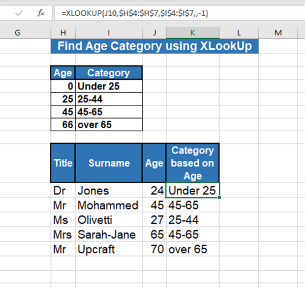
Using the XLOOKUP function to sort people into different age brackets.