It’s a great way to make data entry easier, and to avoid spelling mistakes that lead to inconsistent values when analysing your data. In this blog we will take data validation a step further and look at how to make one drop-down list change its values depending on the choice made in a previous drop-down. We will be working with this sales data as an example:
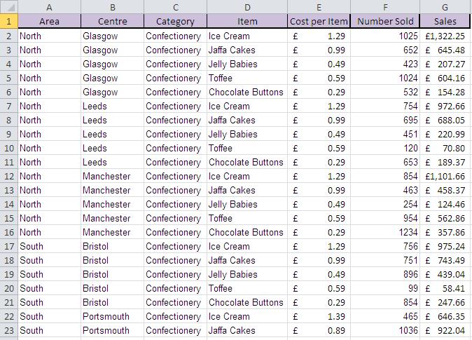
Example data
Let’s assume we have set up data validation on the Area field so that we can choose from North or South:
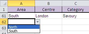
Data validation set up
What we would like is for the drop-down in the Centre field to show us only centres from the North, or only centres from the South, dependent upon our initial choice:
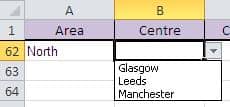
Dependent data
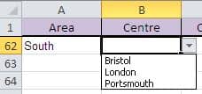
Dependent data
To do this, we have to first set up some named ranges that contain the appropriate values:
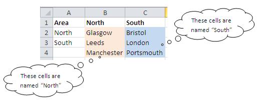
Named ranges
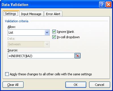
The range names you use must much the values from the first list. When the first value is chosen, this can then be used to create the range name to specify the dependent list. To do this, you must use the INDIRECT function within the Source box of the Data Validation pop-up:
Data validation pop-up
NOTE: When you write the INDIRECT function, you must remember to remove the dollar sign from the row part of the cell reference; otherwise it will always refer to the same cell and will not pick up the correct value for that row.
The INDIRECT function takes the value from column A and turns it into a range name. The values in this range are then used as the source for the data validation list.
Related Blogs
- Calculations on a Filtered List in Excel – In this blog, learn how to create a dropdown filter in your Excel spreadsheets.
- Save Time in Excel with Autofill – Learn how to use the useful tool Autofill. Nicky explains how in the two minute video.
- How Microsoft Excel Can Increase Your Productivity – Billy talks about some of the reasons why Microsoft Excel is so indispensable to productive workplaces in this blog.